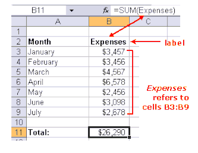
42 accept labels in formulas excel 2013

How to Use Templates and Outlines in Excel 2013 Click the Add button. Enter a name for the view in the Name box. Now go to Include In View and select the settings that you want to include. Click OK. To apply a custom view, click the View tab again, then click Custom Views. Select the name of your view in the Custom Views dialogue box. Click the Show button. How to get ribbon back in Excel 2013 - Stack Overflow The project was developed in Excel 2013. When I opened it, the ribbon tab was gone. I have tried searching for several solutions but haven't found any matching this exact issue. I don't have a tools tab or anything accessible to me. When I click the excel icon top left it says "restore, minimize, close". I have a formula bar, but that's about it.

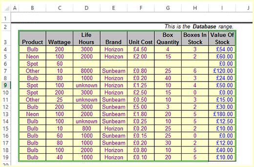
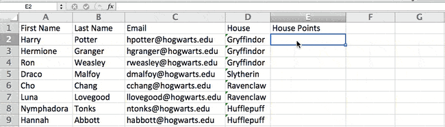
Define and use names in formulas - support.microsoft.com Select Formulas > Create from Selection. In the Create Names from Selection dialog box, designate the location that contains the labels by selecting the Top row,Left column, Bottom row, or Right column check box. Select OK. Excel names the cells based on the labels in the range you designated. Use names in formulas

Accept labels in formulas excel 2013

How to display text labels in the X-axis of scatter chart ... Actually, there is no way that can display text labels in the X-axis of scatter chart in Excel, but we can create a line chart and make it look like a scatter chart. 1. Select the data you use, and click Insert > Insert Line & Area Chart > Line with Markers to select a line chart. See screenshot: 2. Repeat All Item Labels In An Excel Pivot Table - MyExcelOnline You can then select to Repeat All Item Labels which will fill in any gaps and allow you to take the data of the Pivot Table to a new location for further analysis. STEP 1: Click in the Pivot Table and choose PivotTable Tools > Options (Excel 2010) or Design (Excel 2013 & 2016) > Report Layouts > Show in Outline/Tabular Form Excel 2013: Tables - GCFGlobal.org To format data as a table: Select the cells you want to format as a table. In our example, we'll select the cell range A4:D10. Selecting a cell range to format as a table. From the Home tab, click the Format as Table command in the Styles group. Clicking the Format as Table command. Select a table style from the drop-down menu.

Accept labels in formulas excel 2013. Improve your X Y Scatter Chart with custom data labels Luckily the people at Microsoft have heard our prayers. They have implemented a feature into Excel 2013 that allows you to assign a cell to a chart data point label a, in an x y scatter chart.. I will demonstrate how to do this for Excel 2013 and later versions and a workaround for earlier versions in this article. Adding rich data labels to charts in Excel 2013 ... To add a data label in a shape, select the data point of interest, then right-click it to pull up the context menu. Click Add Data Label, then click Add Data Callout . The result is that your data label will appear in a graphical callout. In this case, the category Thr for the particular data label is automatically added to the callout too. Excel- Labels, Values, and Formulas - WebJunction Simple Formula: Click the cell in which you want the answer (result of the formula) to appear. Press Enter once you have typed the formula. All formulas start with an = sign. Refer to the cell address instead of the value in the cell e.g. =A2+C2 instead of 45+57. That way, if a value changes in a cell, the answer to the formula changes with it. IFS Function in Excel 2016, 2013, 2010, and 2007 -- just ... You can add the IFS Function to Excel 2016, 2013, 2010, and 2007. Excel 365 or Excel 2019 introduced a new function called IFS. You can add an IFS function in Excel 2016, 2013 or your copy of Excel 2010, or 2007 with the Excel PowerUps add-in.. This IFS function in Excel 2016 (or earlier) allows you to specify a series of conditions easily in a single function without having to nest several IF ...

How to Print Labels From Excel? | Steps to Print Labels ... Navigate towards the folder where the excel file is stored in the Select Data Source pop-up window. Select the file in which the labels are stored and click Open. A new pop up box named Confirm Data Source will appear. Click on OK to let the system know that you want to use the data source. Again a pop-up window named Select Table will appear. How to Create a Barcode in Excel | Smartsheet How to Create a Barcode in Excel 2013 Download and install a barcode font. Create two rows ( Text and Barcode) in a blank Excel spreadsheet. Use the barcode font in the Barcode row and enter the following formula: ="*"&A2&"*" in the first blank row of that column. Then, fill the formula in the remaining cells in the Barcode row. Excel names and named ranges: how to define and use in ... If your data is arranged in a tabular form, you can quickly create names for each column and/or row based on their labels: Select the entire table including the column and row headers. Go to the Formulas tab > Define Names group, and click the Create from Selection button. Or, press the keyboard shortcut Ctrl + Shift + F3. Excel Formula Not Working - WallStreetMojo 6 Main Reasons for Excel Formula Not Working (with Solution) Reason #1 - Cells Formatted as Text. Reason #2 - Accidentally Typed the keys CTRL + `. Reason #3 - Values are Different & Result is Different. Reason #4 - Don't Enclose Numbers in Double Quotes. Reason #5 - Check If Formulas are Enclosed in Double Quotes.

Use defined names to automatically update a chart range ... Select cells A1:B4. On the Insert tab, click a chart, and then click a chart type. Click the Design tab, click the Select Data in the Data group. Under Legend Entries (Series), click Edit. In the Series values box, type =Sheet1!Sales, and then click OK. Under Horizontal (Category) Axis Labels, click Edit. Add a label or text box to a worksheet You can add labels to forms and ActiveX controls. Add a label (Form control) Click Developer, click Insert, and then click Label . Click the worksheet location where you want the upper-left corner of the label to appear. To specify the control properties, right-click the control, and then click Format Control. Add a label (ActiveX control) How to Wrap Text and Formulas on Multiple Lines in Excel Select a cell and enter text; press and hold Alt.Press Enter and release Alt.For more than two lines of text, press Alt+Enter at each line's end.; Wrap existing text: Select the cell, press F2, place the cursor where you want the line broken.Press and hold Alt.Press Enter and release Alt.; Or, use the Ribbon: Select the cell that contains the text to be wrapped. Excel 2013, Filter not working for all table content ... Excel 2013, Filter not working for all table content. Hi all, Using Excel 2013 I have a table of 566 rows. When applying any filter in any column it only works down to row 468, then it displays rows 469-566 as if unfiltered. When I use Ctrl+A it only highlights data from Row 1-468. If I click on any rows below 468 and press Ctrl+A it highlights ...

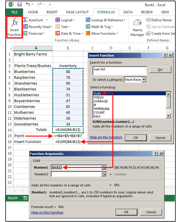
Excel 2016 - How to Use Formulas and Functions To do this, we are going to click Insert Function on the Ribbon under the Formulas tab. Once again, we enter "average of cells" in the "Search for a Function field," then click the Go button. Select Average, then click OK. Excel prompts us for our arguments. The arguments are the cells or values that we want to use to calculate the function.

Enable or Disable Excel Data Labels at the click of a ... Select and to go Insert tab > Charts group > Click column charts button > click 2D column chart. This will insert a new chart in the worksheet. Step 2: Having chart selected go to design tab > click add chart element button > hover over data labels > click outside end or whatever you feel fit. This will enable the data labels for the chart.

How to Print Labels from Excel - Lifewire Choose Start Mail Merge > Labels . Choose the brand in the Label Vendors box and then choose the product number, which is listed on the label package. You can also select New Label if you want to enter custom label dimensions. Click OK when you are ready to proceed. Connect the Worksheet to the Labels

Excel 2013: Label deconfliction in labeled scatter plot ... Bookmark this question. Show activity on this post. In Excel 2013, I am labeling a scatter plot with values from cells. I'd like the labels to not overlap. I can manually move labels, but I've created a filter to automatically create new plots, so I would like the label deconfliction to happen automatically as well.

How to Use the AutoSum Feature in Microsoft Excel 2013 Excel will select a range of adjacent cells for you. If Excel choose the wrong range of cells, just use your mouse to click and drag over the correct range of cells to use in the formula. 2. Click the "AutoSum" button again or press the "Enter" key on your keyboard to accept the formula. 3.

How to use AutoFill in Excel - all fill handle options ... In Excel 2010-2013 click File -> Options -> Advanced -> scroll to the General section to find the Edit Custom Lists… button. Since you already selected the range with your list, you will see its address in the Import list from cells: field. Press the Import button to see your series in the Custom Lists window.

How to Convert a Formula to a Static Value in Excel 2013 Select the cells that contain formulas you want to convert to static values. You can either drag across the cell range, if they're contiguous, or press Ctrl when selecting cells if they are not contiguous. Click Copy in the Clipboard section of the Home tab or press Ctrl + C to copy the selected cells.

Excel Table: Header with formula - Microsoft Community Click in your table, select Design under Table Tools on the ribbon, and then uncheck "Header Row". That should allow you to enter a formula in the cell above your table data. This method can be used when you are willing to sacrifice the "Sort" ability of Header Row after you protect the sheet.

Excel data doesn't retain formatting in mail merge ... Method 1 Use Dynamic Data Exchange (DDE) to connect to the Excel worksheet that contains the data that you want to use. Start Word, and then open a new blank document. Select File > Options. On the Advanced tab, go to the General section. Select the Confirm file format conversion on open check box, and then select OK.

Share :