38 how to insert data labels in excel pie chart

Add or remove data labels in a chart - support.microsoft.com Click the data series or chart. To label one data point, after clicking the series, click that data point. In the upper right corner, next to the chart, click Add Chart Element > Data Labels. To change the location, click the arrow, and choose an option. If you want to show your data label inside a text bubble shape, click Data Callout. excel - Positioning data labels in pie chart - Stack Overflow Sub tester () Dim se As Series Set se = Totalt.ChartObjects ("Inosa gule").Chart.SeriesCollection ("Grøn pil") se.ApplyDataLabels With se.DataLabels .NumberFormat = "0,0 %" With .Format.Fill .ForeColor.RGB = RGB (255, 255, 255) .Transparency = 0.15 End With .Position = xlLabelPositionCenter End With End Sub

c# - Add data labels to excel pie chart - Stack Overflow I am drawing a pie chart with some data: private void DrawFractionChart(Excel.Worksheet activeSheet, Excel.ChartObjects xlCharts, Excel.Range xRange, Excel.Range yRange) { Excel.ChartObject ... Add data labels to excel pie chart. Ask Question Asked 9 years, 11 months ago. Modified 5 years, 11 months ago. Viewed 9k times

How to insert data labels in excel pie chart

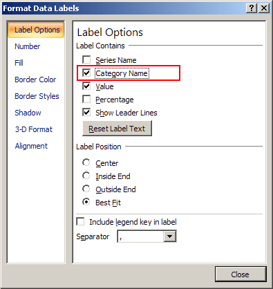
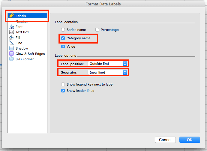
Create a Pie Chart in Excel (In Easy Steps) - Excel Easy Click the + button on the right side of the chart and click the check box next to Data Labels. 10. Click the paintbrush icon on the right side of the chart and change the color scheme of the pie chart. Result: 11. Right click the pie chart and click Format Data Labels. 12. Check Category Name, uncheck Value, check Percentage and click Center. How to Make a Pie Chart in Excel: 10 Steps (with Pictures) 1. Open Microsoft Excel. It resembles a white "E" on a green background. If you would rather make a chart from data you already have, double-click the Excel document that contains the data to open it and proceed to the next section. 2. Click Blank workbook (PC) or Excel Workbook (Mac). How to Create and Format a Pie Chart in Excel - Lifewire To add data labels to a pie chart: Select the plot area of the pie chart. Right-click the chart. Select Add Data Labels . Select Add Data Labels. In this example, the sales for each cookie is added to the slices of the pie chart. Change Colors

How to insert data labels in excel pie chart. How to add or move data labels in Excel chart? - ExtendOffice In Excel 2013 or 2016. 1. Click the chart to show the Chart Elements button . 2. Then click the Chart Elements, and check Data Labels, then you can click the arrow to choose an option about the data labels in the sub menu. See screenshot: In Excel 2010 or 2007. 1. click on the chart to show the Layout tab in the Chart Tools group. See ... Add data labels and callouts to charts in Excel 365 - EasyTweaks.com The steps that I will share in this guide apply to Excel 2021 / 2019 / 2016. Step #1: After generating the chart in Excel, right-click anywhere within the chart and select Add labels . Note that you can also select the very handy option of Adding data Callouts. Add a DATA LABEL to ONE POINT on a chart in Excel All the data points will be highlighted. Click again on the single point that you want to add a data label to. Right-click and select ' Add data label '. This is the key step! Right-click again on the data point itself (not the label) and select ' Format data label '. You can now configure the label as required — select the content of ... Adding data labels to a pie chart - OzGrid Free Excel/VBA Help Forum Re: Adding data labels to a pie chart Yes it doesn't appear via intelli-sense unless you use a Series object. Code Dim objSeries As Series Set objSeries = ActiveChart.SeriesCollection (1) objSeries.HasDataLabels [h4] Cheers Andy [/h4] norie Super Moderator Reactions Received 8 Points 53,548 Posts 10,650 Feb 25th 2005 #9

Excel charts: add title, customize chart axis, legend and data labels Click anywhere within your Excel chart, then click the Chart Elements button and check the Axis Titles box. If you want to display the title only for one axis, either horizontal or vertical, click the arrow next to Axis Titles and clear one of the boxes: Click the axis title box on the chart, and type the text. Office: Display Data Labels in a Pie Chart If you have not inserted a chart yet, go to the Insert tab on the ribbon, and click the Chart option. 3. In the Chart window, choose the Pie chart option from the list on the left. Next, choose the type of pie chart you want on the right side. 4. Once the chart is inserted into the document, you will notice that there are no data labels. How to create a pie chart in Excel Step 1: Highlight the data to chart. Step 2: In INSERT-> select the icon of the pie chart -> choose the type of chart to draw, in this example, select the pie chart 2 - D Pie. Step 3: After selecting the chart type, the pie chart is drawn as shown: - In case you want to change the data on a spreadsheet -> the chart updates itself with that change. Adding data labels to a Pie Chart in VBA - Automate Excel The ultimate Excel charting Add-in. Easily insert advanced charts. Charts List. List of all Excel charts. Adding data labels to a Pie Chart in VBA. Excel and VBA Consulting Get a Free Consultation. VBA Code Generator; VBA Tutorial; VBA Code Examples for Excel; Excel Boot Camp;

Pie of Pie Chart in Excel - Inserting, Customizing, Formatting Inserting a Pie of Pie Chart. Let us say we have the sales of different items of a bakery. Below is the data:-. To insert a Pie of Pie chart:-. Select the data range A1:B7. Enter in the Insert Tab. Select the Pie button, in the charts group. Select Pie of Pie chart in the 2D chart section. How to Add Data Labels to an Excel 2010 Chart - dummies Excel provides several options for the placement and formatting of data labels. Use the following steps to add data labels to series in a chart: Click anywhere on the chart that you want to modify. On the Chart Tools Layout tab, click the Data Labels button in the Labels group. A menu of data label placement options appears: Microsoft Excel Tutorials: Add Data Labels to a Pie Chart To add the numbers from our E column (the viewing figures), left click on the pie chart itself to select it: The chart is selected when you can see all those blue circles surrounding it. Now right click the chart. You should get the following menu: From the menu, select Add Data Labels. New data labels will then appear on your chart: How to add data labels from different column in an Excel chart? Right click the data series in the chart, and select Add Data Labels > Add Data Labels from the context menu to add data labels. 2. Click any data label to select all data labels, and then click the specified data label to select it only in the chart. 3.

Pie Chart in Excel - Easy Excel Tutorial

Pie Chart in Excel | How to Create Pie Chart - EDUCBA Step 1: Do not select the data; rather, place a cursor outside the data and insert one PIE CHART. Go to the Insert tab and click on a PIE. Step 2: once you click on a 2-D Pie chart, it will insert the blank chart as shown in the below image. Step 3: Right-click on the chart and choose Select Data.

How to Data Labels in a Pie chart in Excel 2010 - YouTube

How to insert data labels to a Pie chart in Excel 2013 - YouTube This video will show you the simple steps to insert Data Labels in a pie chart in Microsoft® Excel 2013. Content in this video is provided on an "as is" basi...

Excel 3-D Pie charts - Microsoft Excel 2007

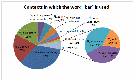
Inserting Data Label in the Color Legend of a pie chart Inserting Data Label in the Color Legend of a pie chart. Hi, I am trying to insert data labels (percentages) as part of the side colored legend, rather than on the pie chart itself, as displayed on the image below. Does Excel offer that option and if so, how can i go about it?

How to Make a Pie Chart in Excel & Add Rich Data Labels to The Chart!

Pie Chart in Excel - Inserting, Formatting, Filters, Data Labels To add Data Labels, Click on the + icon on the top right corner of the chart and mark the data label checkbox. You can also unmark the legends as we will add legend keys in the data labels. We can also format these data labels to show both percentage contribution and legend:- Right click on the Data Labels on the chart.

EXCEL Charts: Column, Bar, Pie and Line

Add Labels with Lines in an Excel Pie Chart (with Easy Steps) To enables the data labels on the pie chart, Click on the Pie Chart first. Then click on the plus icon at the top-right corner of the pie chart. Now select Data Labels in the Chart Elements list. After that, you will see a variety of data labels position option such as, Center Inside End Outside End Best Fit Data callout

Excel 3-D Pie Charts

How to Make a Pie Chart in Excel & Add Rich Data Labels to The Chart! 2) Go to Insert> Charts> click on the drop-down arrow next to Pie Chart and under 2-D Pie, select the Pie Chart, shown below. 3) Chang the chart title to Breakdown of Errors Made During the Match, by clicking on it and typing the new title.

How to create pie of pie or bar of pie chart in Excel?

Edit titles or data labels in a chart - support.microsoft.com The first click selects the data labels for the whole data series, and the second click selects the individual data label. Right-click the data label, and then click Format Data Label or Format Data Labels. Click Label Options if it's not selected, and then select the Reset Label Text check box. Top of Page

How to Create a Pie Chart in Excel | Smartsheet

Possible to add second data label to pie chart? - Excel Help Forum You get one data label per plotted point. I think you could use the first trick in this page of Andy Pope's, and make the pie in front the same size as the one in back, and use one pie for the outside labels and the other for the inside labels. - Jon ------- Jon Peltier, Microsoft Excel MVP Peltier Technical Services Tutorials and Custom Solutions

How to Make a Pie Chart in Excel & Add Rich Data Labels to The Chart!

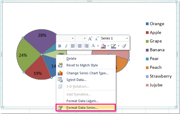
Chart Legend / Data Labels In Pie Chart - MrExcel Message Board Jun 6, 2009. #3. Add the data labels. Then, right click on any data label to select all the data labels for that series and select Format Data Labels... From the Label Options tab, in the Label Contains section, select the 'Series Name' checkbox. The above applies to Excel 2007. Excel 2003 supports the same capability though the dialog box ...

Microsoft Excel Tutorials: Add Data Labels to a Pie Chart

How to Create a Pie Chart in Excel - Smartsheet Enter data into Excel with the desired numerical values at the end of the list. Create a Pie of Pie chart. Double-click the primary chart to open the Format Data Series window. Click Options and adjust the value for Second plot contains the last to match the number of categories you want in the "other" category.

Creating Pie Chart and Adding/Formatting Data Labels (Excel) - YouTube

How to Create and Format a Pie Chart in Excel - Lifewire To add data labels to a pie chart: Select the plot area of the pie chart. Right-click the chart. Select Add Data Labels . Select Add Data Labels. In this example, the sales for each cookie is added to the slices of the pie chart. Change Colors

How to Add percentage data Labels in Excel Bar chart, 1

How to Make a Pie Chart in Excel: 10 Steps (with Pictures) 1. Open Microsoft Excel. It resembles a white "E" on a green background. If you would rather make a chart from data you already have, double-click the Excel document that contains the data to open it and proceed to the next section. 2. Click Blank workbook (PC) or Excel Workbook (Mac).