43 pie chart excel labels

Formatting data labels and printing pie charts on Excel for Mac 2019 ... Here's a work around I found for printing pie charts. Still can't find a solution for formatting the data labels. 1. When printing a pie chart from Excel for mac 2019, MS instructions are to select the chart only, on the worksheet > file > print. Excel is supposed to print the chart only (not the data ) and automatically fit it onto one page. Excel custom pie chart labels - Microsoft Community Excel custom pie chart labels I have a data set like this (basically form output): I want to use a pivot table to make a pie chart out of this. I want each of the pieces of the pie to contain the number of entries and between parentheses the percentage. So in the "Yes" piece, there should be '3 (33%)'.

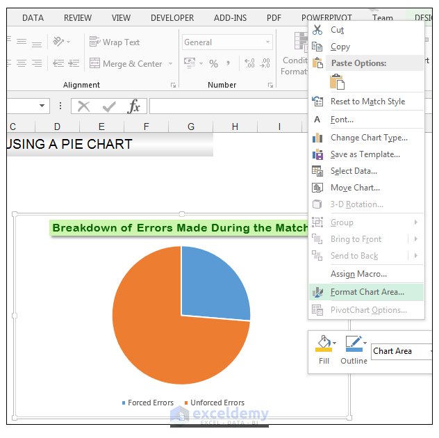
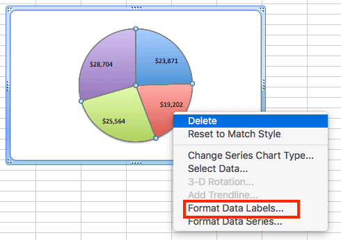
How to Create and Format a Pie Chart in Excel - Lifewire Select the plot area of the pie chart. Right-click the chart. Select Add Data Labels . Select Add Data Labels. In this example, the sales for each cookie is added to the slices of the pie chart. Change Colors When a chart is created in Excel, or whenever an existing chart is selected, two additional tabs are added to the ribbon.

Pie chart excel labels

How to plot a pie chart in Excel | Basic Excel Tutorial NOTE. 1. On your computer, open the worksheet you want to create a pie chart. 2. In your spreadsheet, select the range of data you want to use for your pie chart. 3. On the main menu ribbon, click on the Insert tab. 4. Here you will see different types of charts, click on the Pie chart icon drop-down arrow. › data-series-data-points-dataUnderstanding Excel Chart Data Series, Data Points, and Data ... Sep 19, 2020 · Percentage labels are commonly used for pie charts. Data Series : A group of related data points or markers that are plotted in charts and graphs. Examples of a data series include individual lines in a line graph or columns in a column chart. Understanding Excel Chart Data Series, Data Points, and Data Labels 19.09.2020 · Numeric Values: Taken from individual data points in the worksheet.; Series Names: Identifies the columns or rows of chart data in the worksheet. Series names are commonly used for column charts, bar charts, and line graphs. Category Names: Identifies the individual data points in a single series of data.These are commonly used for pie charts.

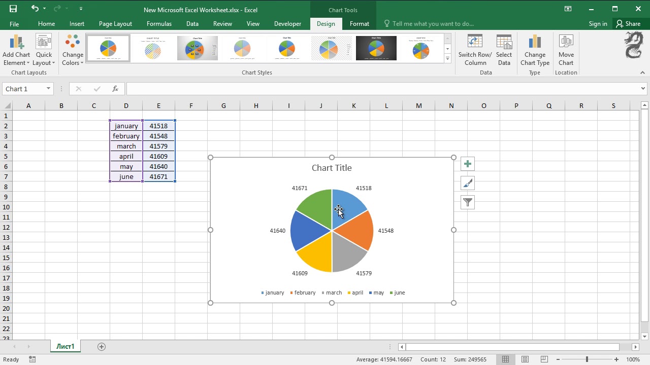
Pie chart excel labels. How to Rotate Pie Chart in Excel? - WallStreetMojo Move the cursor to the chart area to select the pie chart. Step 5: Click on the Pie chart and select the 3D chart, as shown in the figure, and develop a 3D pie chart. Step 6: In the next step, change the title of the chart and add data labels to it. Step 7: To rotate the pie chart, click on the chart area. How to Create Pie Charts in Excel (In Easy Steps) Select the pie chart. 9. Click the + button on the right side of the chart and click the check box next to Data Labels. 10. Click the paintbrush icon on the right side of the chart and change the color scheme of the pie chart. Result: 11. Right click the pie chart and click Format Data Labels. 12. Answered: Excel 3-Activity 2 - Imbedded Pie… | bartleby Question. Transcribed Image Text: Excel 3 - Activity 2 - Imbedded Pie Charts 1. Open the Excel 3 Activity 2 Weekly Sales Pie Chart file from the shared drive. 2. Save the file as 21 Activity Activity2 3. to your student drive in your Excel 3 folder. 4. Update the header and footer in class format. 5. Everything You Need to Know About Pie Chart in Excel How to Make a Pie Chart in Excel. Start with selecting your data in Excel. If you include data labels in your selection, Excel will automatically assign them to each column and generate the chart. Go to the INSERT tab in the Ribbon and click on the Pie Chart icon to see the pie chart types. Click on the desired chart to insert.

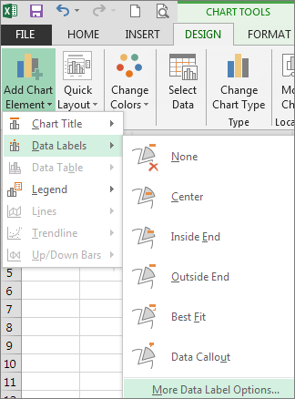
Multiple data labels (in separate locations on chart) You can do it in a single chart. Create the chart so it has 2 columns of data. At first only the 1 column of data will be displayed. Move that series to the secondary axis. You can now apply different data labels to each series. Attached Files 819208.xlsx‎ (13.8 KB, 263 views) Download Cheers Andy Register To Reply Pie Chart Best Fit Labels Overlapping - VBA Fix I created attached Pie chart in Excel with 31 points and all labels are readable and perfectly placed. It is created from few clicks without VBA using data visualization tool in Excel. Data Visualization Tool For Excel Data Visualization Tool For Google Sheets It has auto cluttering effect to adjust according to your data size. Add or remove data labels in a chart - support.microsoft.com Click the data series or chart. To label one data point, after clicking the series, click that data point. In the upper right corner, next to the chart, click Add Chart Element > Data Labels. To change the location, click the arrow, and choose an option. If you want to show your data label inside a text bubble shape, click Data Callout. Edit titles or data labels in a chart - support.microsoft.com On a chart, click the label that you want to link to a corresponding worksheet cell. On the worksheet, click in the formula bar, and then type an equal sign (=). Select the worksheet cell that contains the data or text that you want to display in your chart. You can also type the reference to the worksheet cell in the formula bar.

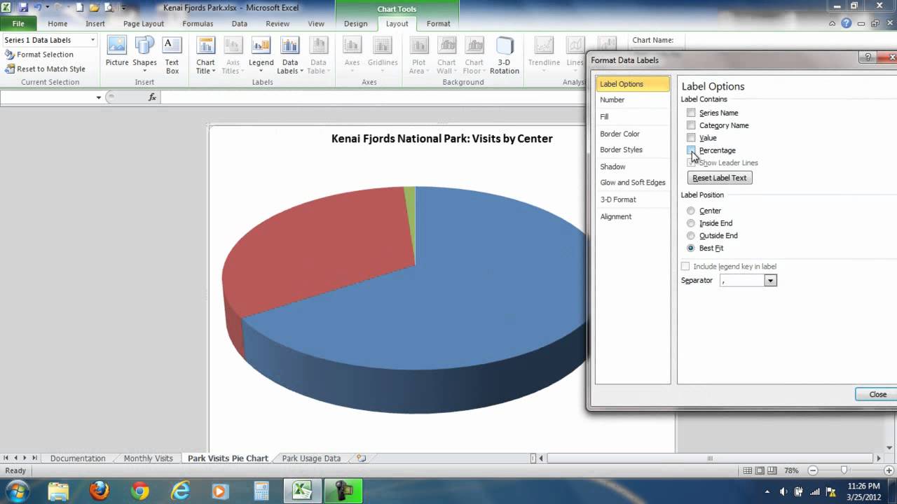
I cannot change the default label positions on a pie chart. The option ... Under Add chart element/Data labels, I can only choose "none", "show" or "callout". When I go to "More data label ... Pie charts should have several options: Center, Inside End, Outside End, and Best Fit. ... I've searched extensively for an answer to this problem and the only response seems to be that excel doesn't offer this option for all ... c# - Add data labels to excel pie chart - Stack Overflow I am drawing a pie chart with some data: private void DrawFractionChart(Excel.Worksheet activeSheet, Excel.ChartObjects xlCharts, Excel.Range xRange, Excel.Range yRange) { Excel.ChartObject ... Add data labels to excel pie chart. Ask Question Asked 9 years, 9 months ago. Modified 5 years, 10 months ago. Viewed 9k times › graphs › pie-chartsFree Pie Chart Maker - Create Online Pie Charts in Canva Pie chart maker features. With Canva’s pie chart maker, you can make a pie chart in less than a minute. It’s ridiculously easy to use. Start with a template – we’ve got hundreds of pie chart examples to make your own. Then simply click to change the data and the labels. How to Insert Axis Labels In An Excel Chart | Excelchat We will go to Chart Design and select Add Chart Element Figure 6 - Insert axis labels in Excel In the drop-down menu, we will click on Axis Titles, and subsequently, select Primary vertical Figure 7 - Edit vertical axis labels in Excel Now, we can enter the name we want for the primary vertical axis label.

33 How To Label Pie Chart In Excel - Labels Design Ideas 2020

Chowhound Thank you for making Chowhound a vibrant and passionate community of food trailblazers for 25 years. We wish you all the best on your future culinary endeavors.

Creating a 3D Pie Chart in Excel Vid.wmv - YouTube

excel - Positioning data labels in pie chart - Stack Overflow Sub tester () Dim se As Series Set se = Totalt.ChartObjects ("Inosa gule").Chart.SeriesCollection ("Grøn pil") se.ApplyDataLabels With se.DataLabels .NumberFormat = "0,0 %" With .Format.Fill .ForeColor.RGB = RGB (255, 255, 255) .Transparency = 0.15 End With .Position = xlLabelPositionCenter End With End Sub

How to Create Excel Pie Charts & Add Rich Data Labels to The Chart!

spreadsheeto.com › pie-chartHow To Make A Pie Chart In Excel: In Just 2 Minutes [2022] How To Make A Pie Chart In Excel. In Just 2 Minutes! Written by co-founder Kasper Langmann, Microsoft Office Specialist. The pie chart is one of the most commonly used charts in Excel. Why? Because it’s so useful 🙂. Pie charts can show a lot of information in a small amount of space. They primarily show how different values add up to a whole.

Excel 3-D Pie Charts

Pie Chart in Excel | How to Create Pie Chart | Step-by-Step Guide Chart In this way, we can present our data in a PIE CHART makes the chart easily readable. Example #2 – 3D Pie Chart in Excel. Now we have seen how to create a 2-D Pie chart. We can create a 3-D version of it as well. For this example, I have taken sales data as an example. I have a sale person name and their respective revenue data.

r - labels on the pie chart for small pieces (ggplot) - Stack Overflow

Excel 2010 pie chart data labels in case of "Best Fit" Based on my tested in Excel 2010, the data labels in the "Inside" or "Outside" is based on the data source. If the gap between the data is big, the data labels and leader lines is "outside" the chart. And if the gap between the data is small, the data labels and leader lines is "inside" the chart. Regards, George Zhao TechNet Community Support

How to display percentage labels in pie chart in Excel - YouTube

Pie of Pie Chart in Excel - Inserting, Customizing, Formatting Inserting a Pie of Pie Chart. Let us say we have the sales of different items of a bakery. Below is the data:-. To insert a Pie of Pie chart:-. Select the data range A1:B7. Enter in the Insert Tab. Select the Pie button, in the charts group. Select Pie of Pie chart in the 2D chart section.

How to rotate the slices in Pie Chart in Excel 2010 - YouTube

Pie Chart in Excel | How to Create Pie Chart - EDUCBA Pie Chart in Excel is used for showing the completion or main contribution of different segments out of 100%. It is like each value represents the portion of the Slice from the total complete Pie. For Example, we have 4 values A, B, C and D.

How to Show Percentages in Stacked Bar and Column Charts in Excel

How to show percentage in pie chart in Excel? - ExtendOffice Please do as follows to create a pie chart and show percentage in the pie slices. 1. Select the data you will create a pie chart based on, click Insert > I nsert Pie or Doughnut Chart > Pie. See screenshot: 2. Then a pie chart is created. Right click the pie chart and select Add Data Labels from the context menu. 3.

SQL & BI Learning: Pie Chart with data labels outside in ssrs

How to make a pie chart in Excel - ablebits.com 12.11.2015 · How to show percentages on a pie chart in Excel. When the source data plotted in your pie chart is percentages, % will appear on the data labels automatically as soon as you turn on the Data Labels option under Chart Elements, or select the Value option on the Format Data Labels pane, as demonstrated in the pie chart example above.. If your source data are …

How to Create a Pie Chart in Excel | Smartsheet

How to Create a Pie Chart in Excel | Smartsheet To create a pie chart in Excel 2016, add your data set to a worksheet and highlight it. Then click the Insert tab, and click the dropdown menu next to the image of a pie chart. Select the chart type you want to use and the chosen chart will appear on the worksheet with the data you selected.

Python matplotlib Pie Chart

How To Make A Pie Chart In Excel: In Just 2 Minutes [2022] When you first create a pie chart, Excel will use the default colors and design.. But if you want to customize your chart to your own liking, you have plenty of options. The easiest way to get an entirely new look is with chart styles.. In the Design portion of the Ribbon, you’ll see a number of different styles displayed in a row. Mouse over them to see a preview:

Insert a pie chart in Excel - Excel

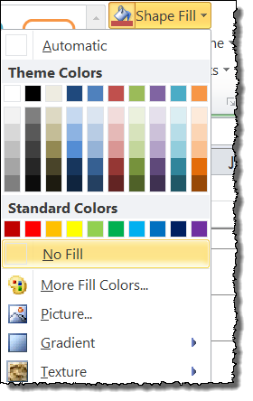
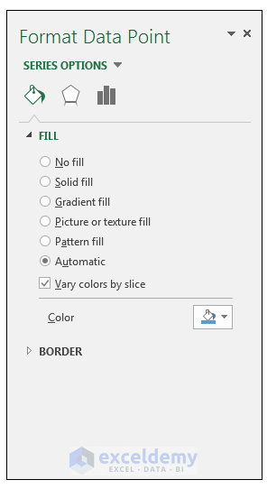
How to eliminate zero value labels in a pie chart - MrExcel Message Board However you can hide the 0% using custom number formatting. Right click the label and select Format Data Labels. Then select the Number tab and then Custom from the Categories. Enter. 0%; [White] [=0]General;General. in the Type box. This will set the font colour to white if a label has a value of zero.

410 How to display percentage labels in pie chart in Excel 2016 - YouTube

› 07 › 09Rotate charts in Excel - spin bar, column, pie and line ... Jul 09, 2014 · I think 190 degrees will work fine for my pie chart. After being rotated my pie chart in Excel looks neat and well-arranged. Thus, you can see that it's quite easy to rotate an Excel chart to any angle till it looks the way you need. It's helpful for fine-tuning the layout of the labels or making the most important slices stand out. Rotate 3-D ...

How to Make a Pie Chart in Excel & Add Rich Data Labels to The Chart!

Only Display Some Labels On Pie Chart - Excel Help Forum Only Display Some Labels On Pie Chart. I have a pie chart that contains over 50 categories (Yes, I know pie charts shouldn't be used for that many things) but I want to only display labels for maybe the top 5 values or any label with a value >10. This is because there are a few standout values but I want all the other values to remain in the ...

Share :